A Hitchhikers Guide to Data Science....

This article is supposed to be a rough guide to all aspiring data scientists. It is a whistle stop tour of all the necessary steps to create a data science project, including the tools and practical tips. 


STEP No1 --> ASK THE QUESTION

Data science is all about asking the right question,, formulating a hypothesis. For our example: "Could you predict the rating of a movie before it hits the theatres, or even better – before the movie is even made?" This is of course a holy grail of any Hollywood or Bollywood studioand not an easy question to answer. Let’s assume it can be done, let’s create a plan of action and describe the whole process, covering some pitfalls and mistakes that can be made or avoided. You can only become an expert if you have done all the possible mistakes and learned from them ;-) . 


STEP No2 --> GET THE DATA
There are 3 ways you could find data out there: 1) Buy it (last resort). 2) Find it, plenty of free datasets out there (some free collections  here and here). 3) Scrape it from websites. Data scraping is is the most interesting option. There is tonnes of data just waiting for you to grab it with a program that automates the entire procedure. Scraping is a must have tool in the arsenal of every data scientist. 


BUT WHAT DATA ?

This is the part of data science that is more of an art than a science. What data and from where? The quality and the content of your data set is crucial - it is called features engineering. An easy answer would be to get as much data as you can. Quite ofter it is not the best strategy though, as the data acquisition can be expensive and/or add noise to your dataset.As rule of thumb, ask yourself “what would one need to be able to predict a rating of a movie?” .For example I would base my analysis on parameters like: director, lead actor(s), writer, runtime, genre, country of origin, estimated budget and production company. Watch out to never include features that have a priori knowledge of the result. This introduces a bias and it is called data leakage, see more here.Consequently your model would perform brilliantly on your datasets but it would be useless in real life (a sign of data leakage is a very successful predictive capability for noisy and difficult to predict datasets like e.g. stock market). 

SCRAPING DATA

To scrape the data I use the web library from pattern module. This python module is perfect for scraping so get the hang of it here. The scraping code I created is here and you can use it as a guide for your own projects as it very well commented. Feel free to ask me any question in the comments below. Web scraping is more an art than a science with lots of trial and error involved but it is a very good exercise of python, HTTP requests and DOM manipulation. I am sure you will love it if you practice enough. When you learn how to scrape effectively only the sky is the limit in terms of the data you can obtain. If you are bored though you could use some auto-scrape tools like import.io, although getting your hands dirty is the most effective way always. Word of caution: Do not overdo it with scraping. Some websites will consider this an attack and block your IP. For some others it is illegal. Proceed with caution, have brakes between scraping sessions, use ethics in what you scrape. Play the video below to see how scraping looks into your Mac OS terminal.



Beautiful isn't it?

When you have all your scraped data organised in your python lists (in our case we scraped titles, genres, directors, first_actor, second_actor, runtimes and ratings lists) it is time to create a pandas DataFrame. To do that you will need to invoke these very elegant python commands below:

titles, genres, directors, first_actors, second_actors, runtimes, ratings =zip(*data)

data = pd.DataFrame({'title': titles, 'genres': genres, 'director':directors, 'first_actor':first_actors, 'second_actor':second_actors, 'runtime': runtimes, 'rating': ratings})

print data

These commands allow you to build separate lists from the scraped list of lists (unzip the lists). Then you use these lists to build the columns of your panda dataframe. Using pandas helps you manipulate the data. Data manipulation is a must have skill. Best book out there to learn pandas is Python for data analysis which I definitely recommend.

STEP No 3: DATA WRANGLING OR MUNGING

So you got the data. Congrats. This is where your real job as a data scientist starts. You will spend most of your time cleaning, transforming and doing all the other janitor tasks you need in order to have your data shiny and clean ( data janitor is a less sexy way to say that I am a data scientist but it is not far from the truth). You may download the dirty data I have scraped from IMDB site here and try to clean it.

To start cleaning your data you need to take a look into them and see what is going on. Look into the numerical variables first and check for outliers with the DataFrame.describe() function. You will be looking for data points with high std or max that don't make any sense, for example runtime of a movie with 0 value as a minimum is probably an error in your data. If your numerical variables have high standard deviation created by few data points then your model might be vulnerable to that. To fix it you you need a function that weights the data points according to their distance from mean and reduces the effect if they are too distant (see Huber's weight function here). Runtime has "mins." attached. You should remove mins and keep only the number. Genres are also in a type of [Drama, Action, Fantasy] list. So you should remove the brackets and split them to the comma and use a 0 or 1 for every genre for every movie. These are common munging jobs and should become your second nature. I provide a file for these data munging jobs here and the ipython notebook will be provided soon.

Check your categorical variables with describe() function as well. You could see that most frequent director in our dataset is Woody Allen in 23 movies, most frequent first actor is Nicolas Cage seen in 34 movies and most frequent second actor Samuel Jackson seen in 17 movies.

You should also check for missing values. How would you handle missing values? One way is to drop the rows that have them and dropna() function is a convenient pandas function. Or you may try to fill the missing values with 0 or the mean value for the category but you might introduce noise with that. Another way is to try to predict the missing value with separate models that predict it based on the other variables of the model. There is no rule about what you should do with missing values. If the missing values are more than say 60% you might as well drop the column as a whole but in some cases like when you try to predict outliers that are rare this column might be important.

Arduous trial and error is the key since your are a data janitor after all (sounds less sexy the sexiest job of the 21st century, doesn't it? That's the catch... If something sounds too good to be true then there is a catch, keep this in mind when you build your models also... ). One of the best tutorials for data wrangling with pandas can be found here.

Exploratory data analysis (EDA) is the next step in your data wrangling process where you try to create an interface between the data and your brain which is very good at pattern recognition when it is presented with visualisations. So you create visualisations that can help you feel the data. This is done with histograms and scatter plots for starters. Let's see histograms for ratings and runtimes along with a scatter plot for these two variables.













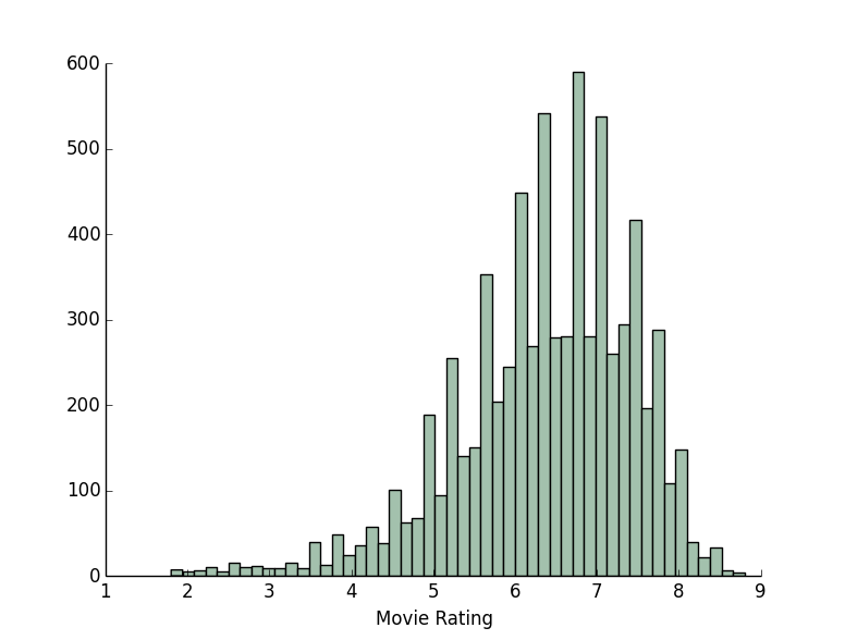
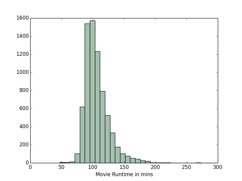
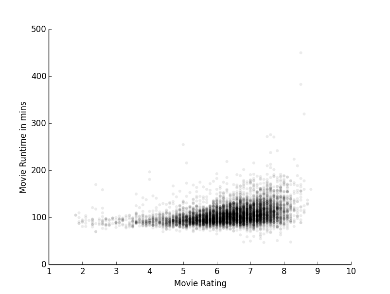
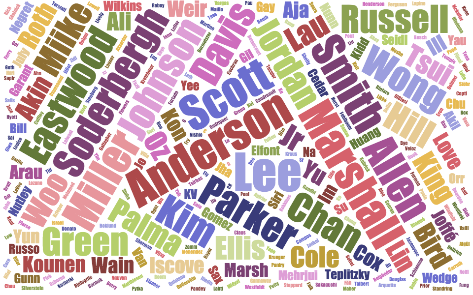
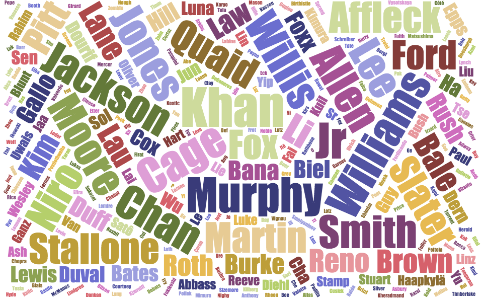
You now have an image of the distribution of these variables. Want to check the categorical variables? Remove the first names of the first actors and make a word cloud out of these. In order to get the surnames you can use a list comprehension where you ask for the last element in a pythonic way [-1] for every full name, split in two by ',' in the list of directors full names. You could use two nice word cloud tools here and here. Want to create a heatmap? Use this tool.

surnames = [x.split(' ')[-1] for x in data.director]

Word cloud of directors surnames



Word cloud of first actors surnames



Let's keep on playing with our data. You might have noticed that there are some directors that like playing in their movies. How would you find that? You would need to get the rows where director's full name is the same like first actor's name and then count these values and sort them to descending order. Easy to do with pandas (string manipulation in pandas is so nice..). So after a few lines of code you get the result below showing the director's name and how many movies she has starred as a first actor also.



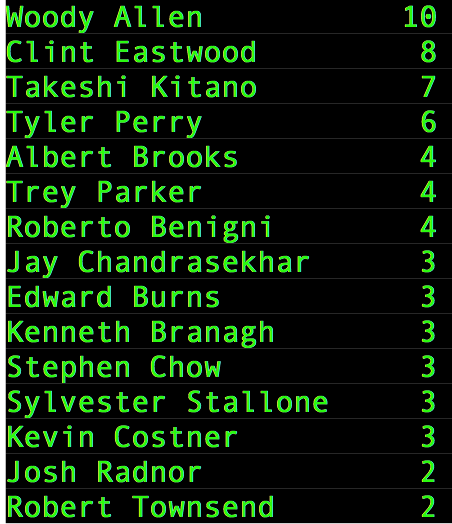
Interesting. Digging a bit deeper you might also notice that there are another 106 movies where the first actor seems to share the same surname with the director. This accounts for 1.4% in our dataset which is not enough to make a meritocracy claim for bias in actors choice :-)

Which are the actors that have participated in movies with more than 8.5 rating? You could keep on doing graphs for possible connections between actors and directors to find possible clusters and many, many more things. Sometimes it is nice to perform an initial cluster analysis of your dataset pretending it was unlabeled, although it is not. You might get some “aha” moments by doing so. For now let's close the chapter of our exploratory data analysis and let’s move on towards creating a model. 


STEP No3--> Create a model

After spending so much time cleaning the data let's go back to the original question. "Can you predict the rating of a movie before it hits the theaters?". We have got the data on titles, runtime, actors, directors and genres and we want to predict IMDB rating. This sounds like a classification job. How many classes? Our dataset has ratings of floating point numbers format to the first decimal which makes our classification job a bit difficult (around 100 classes from 0.0 to 10.0). Let's lower the classes number from 100 to 10 with the following line of code.

data['rating_class']= data.rating // 1

From now on a rating of >=7.6 would belong to 8 class, a rating of <=7.4 would belong to a 7 class etc. Then we should look into the the data a bit further. We have a continuous numerical variable, the runtime, and genre - director - first actor - second actor which are categorical variables. The genre has got a limited number of categories but what is going on with directors? There 3570 different directors in 7279 movies so in order to add this feature to your features matrix you need a 7279 rows X 3570 columns extra space ( a column for every separate name with 1 or 0 for the director of the movie). By doing that also for first & second actor and title of the movie you get a features matrix of 7279 rows x 18271 columns. WT* ?

This is a common characteristic of all the real data science problems. Too many variables, too many dimensions. Have you ever heard about the Curse of Dimensionality? If you want to calculate similarities in huge number of dimensions you would never find a close neighbour because the distances are always very high. Moreover huge matrices mean long computational times for models to be built and too much noise.

Solution? Compress the dimensions by 1) creating subgroups with the most frequent categories and naming the rest other 2) removing the categorical variable that has always the same value so it does not convey any info 3) performing principal component analysis and reducing the dimensions but keep 95% of the variance of the original data. 4) If you are dealing with a dataset where the Zipf's law is valid then you could use the hashing trick to compress your dimensions

In our case we will try to further categorise the categorical variables we have so that there is fewer categories. For every director we will create an average imdb rating for all her movies and categorise all directors according to this (so that every director will be categorised into a matrix of 10 columns with values from 1-10 and cell value of 1 to his average rating and 0 for all the other values). We will do the same with every first and second actor. So instead of thousands of categories we will now have about 30 extra only. Good. But there is a problem in this model. A problem that you will step into very often in your work as data janitor - features engineering. Sometimes you incorporate features that have already a "glimpse of the future" information incorporated. By taking the average per director rating we already incorporated the info about the final prediction which is the movie rating. This is generally a mistake and in this case your model will perform well in your test data and you will be happy till you deploy it in real life and then be super surprised how mediocre it will perform. If you see something like that from now on (good performance in test sets, bad in real life) you will have a hint of what might have happened. Believe me; it is not always as obvious as in this example.

CHOOSE THE RIGHT ALGORITHM --> SIMPLER IS ALWAYS BETTER

For the sake of this exercise we will forget about this mistake and we will move on with our model creation. What algorithm will you choose to build a classification model? Logistic regression (with one vs all)? Support vector machines? Decision trees ? Random forests? Neural networks? Every algorithm has its advantages and disadvantages and the algorithm of choice depends on many variables: do you want insight on the factors affecting the algorithm or not? Do you want it to be performing real time or not? Does it need to be retrained every time a new data point is created or not? Does it need to have all data points on memory or not? These are all very subtle matters that have to be taken into account before choosing an algorithm. In this example I want to use decision trees because they are perfect in handling categorical along with numerical variables in our case the genres, actors, directors and runtime data. The decision trees are also very good in getting insights from our data for example which features are important and convey information (reduce entropy to be accurate) in order to get a guide on what features to keep on collecting (and make the company managers happy as they love insights into what keeps their customers). They are also very fast. Facebook ad machine is powered by decision trees. Fast - insightfull - cheap computationally. On the downside they tend to overfit your data so you need to prune them or reduce the max depth a priori. Everything comes at a price. But you should always start cheap and dirty, get insights on what drives the model and then scale up in complexity, if necessary.

I am going to use python scikit learn for this analysis because I like getting my hands dirty with programming my own code. If you want more easy solutions you can use BimML.com or monkeylearn.com for DIY machine learning. Do not take me wrong: these solutions can be powerful if used as an API when you know what you are doing. They are useful if you want to bootstrap your machine learning startup for example but in general you should know what you do. There is no such thing as machine learning in a super shiny, easy to use give me your data - will give you predictions package. (All opinions here are personal, feel free to comment at the end of this article).

I have prepared the data for the scikit learn which you can get here and follow the recipe below to get the same (or almost the same due to cross validation randomness) results

data = pd.read_csv('data_for_model.csv')

X = data.iloc[:, 1:-1].values
y = data.iloc[:, -1].values

from sklearn import metrics 
from sklearn.cross_validation import train_test_split
from sklearn.tree import DecisionTreeClassifier 

Xtrain, Xtest, ytrain, ytest = train_test_split(X, y, random_state=0) 

clf = DecisionTreeClassifier(max_depth= 5) 
clf.fit(Xtrain, ytrain)
ypred = clf.predict(Xtest)

print metrics.classification_report(ytest, ypred)

Basically what you are doing here is getting your features and classes matrices for the model from your dataframe with the .values command and then split your data into train and test parts and invoke a Decision Tree Classifier estimator. You then fit the classifier - estimator to the train data and use the trained model to predict classes for the test data. You then use the metrics module to get a classification report and a plot for the confusion matrix which should look like the ones below:









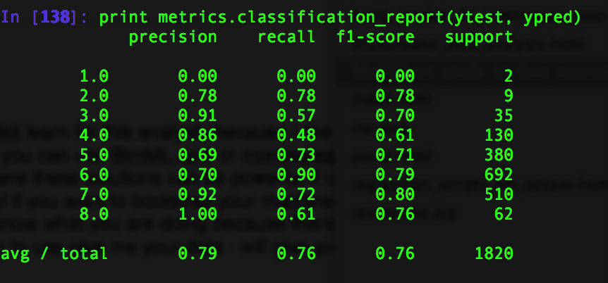
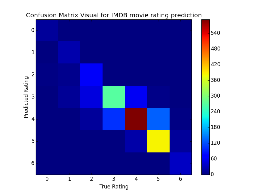
Overall the model did well! Precision of 79% and F1 score of 76% would say not bad at all. But remember that we are using variables that are biased towards the classes like the mean rating of a director for all his movies and the same for actors. One could also comment that we should have done a multi fold cross validation and maybe perform a grid search for the best parameters for our estimator. Or explain what the visualisation of the tree in our decision tree graph means (take a look at the pdf file here). These are important questions and ideas for following posts of course....

Let's have some fun and try to predict the IMDB rating for movies coming out to the cinema soon (the date this article was written is the 13th of October 2014).

Movie: Tomorrowland. Predicted rating class = 7 (meaning IMDB rating above 7 but below 8)

Movie: Focus. Predicted rating class = 6.

Movie: Sex Ed. Predicted rating class = 8. Interesting.

Playing with the data, you can extract some trivia facts, i.e. some movie studios try to team up less known directors with popular actors to increase their chances of success. George Clooney has an average IMDB rating as a first actor of 6. :-) Some actors, like Will Smith have better average rating as second actors rather than first. Interesting stuff. 

Now you have a better grasp of your data, features engineering process and model creation. Time to iterate. Need to get more data or create a better model? This is a question worthy of another post because it is the famous bias - variance trade-off. If you know how to handle this trade-off, you can save your company tonnes of money by using better models and not asking for more data which is always costly.

Hope this article gave you food for thought. Share your throughts in the comments section below.

Back to home »

comments powered by Disqus